Contents
- Bloch's Theorem and the Periodic Potential
- Kronig–Penney Model: Setup and Wavefunctions
- Boundary Conditions and the 4×4 Secular System
- Transfer-Matrix Solution
- The Band-Gap Dispersion Relation
- Physical Interpretation of Band Gaps
- The 1D Hydrogen Chain: Coulomb Tails
- Whittaker Functions and the Coulomb Solution
- Transfer-Matrix Formulation for the H-Chain
- Comparison and Physical Consequences
§1 Bloch's Theorem and the Periodic Potential
Any one-dimensional crystalline solid can be modelled by a Hamiltonian whose potential is periodic with lattice constant $d = a + b$, where $a$ is the width of the "well" region (or the spacing between atoms) and $b$ is the width of the barrier. The central result governing the eigenstates of such a system is Bloch's theorem:
where $k$ is the crystal momentum (Bloch wavevector) and $n$ is the band index. Equivalently, the wavefunction satisfies the quasi-periodicity condition
The factor $e^{ikd}$ is a pure phase, so $|k|$ is restricted to the first Brillouin zone $k \in [-\pi/d,\, \pi/d]$. In one dimension this interval is compact, and the dispersion relation $E_n(k)$ is a multi-valued function of $k$ — the band structure. Band gaps open at the zone boundaries $k = \pm\pi/d$ and, more subtly, at $k = 0$ for higher bands, wherever Bragg reflection is resonant.
§2 Kronig–Penney Model (unbounded case): Setup and Wavefunctions
The Kronig–Penney potential consists of square barriers of height $V_0$ and width $b$, separated by wells of width $a$. as we see below:
Acourdingly, we define two wavevectors for the unbounded electron case as follows:
valid for the upper-barrier regime $E > V_0$. Inside the well region $0 \le x \le a$, the wavefunction is a superposition of left- and right-travelling plane waves:
and inside the barrier $-b \le x \le 0$, the wavefunction is an exponentially growing/decaying pair:
For consistency with Bloch's theorem, we express the Bloch-periodic parts $u_{nk}(x)$ explicitly:
§3 Boundary Conditions and the 4×4 Secular System
Continuity of $\psi$ and $\psi'$ at $x = 0$ and the Bloch condition at $x = a$ (linked back to $x = -b$) yields four linear constraints. Continuity at $x = 0$:
Bloch-shifted continuity at $x = a \leftrightarrow x = -b$:
Casting these four conditions as a matrix equation $\mathbf{M} \begin{pmatrix} A & B & C & D \end{pmatrix}^T = 0$, a non-trivial solution requires:
where the $4\times 4$ matrix $\mathbf{M}$ is:
The determinant can be evaluated by cofactor expansion. Defining the auxiliary quantities $S$ and its factored form as follows (denoting the full determinant $\Delta$), one arrives after careful algebra at the central dispersion relation — derived more elegantly below via the transfer matrix.
§4 Transfer-Matrix Solution, for the bounded case $E < V_0$
To solve the other case, where the electron states in the barrier regin are below the energy barrier $V_0$, we use a more refined method, called the transfer-matrix method, it is a far more systematic alternative to direct determinant evaluation. It expresses the amplitudes $(A, B)$ in one unit cell in terms of those in the next, and enforces Bloch's theorem by demanding the transfer matrix $\mathbf{T}$ has eigenvalues $e^{\pm ikd}$.
4.1 Propagation and Connection Matrices
Within each region we define a state vector $\Omega(x)$ whose columns are the two independent solutions evaluated at $x$, together with their derivatives. For the well region:
For the barrier region (with $k_2$ real and positive for $E < V_0$):
4.2 Constructing the Unit-Cell Transfer Matrix
Continuity at the well–barrier interface $x = 0$:
Similarly, at the barrier–well interface $x = -b$ (and using Bloch periodicity to link to the next cell):
Similarly, at the well interface $x = a$ (and using Bloch periodicity to link to the next cell):
The full unit-cell transfer matrix $\mathbf{T}$ maps amplitudes across one period:
4.3 Eigenvalue Condition and Bloch's Theorem
Bloch's theorem demands:
Since $\mathbf{T_H}$ is a real $2\times 2$ matrix with $\det \mathbf{T} = 1$ (it is symplectic — the Wronskian of the Schrödinger equation is conserved), its eigenvalues are $e^{\pm ikd}$ and the characteristic equation reduces to:
This is the key insight of the transfer-matrix method: the entire band structure is encoded in the trace of a $2\times 2$ matrix. If $|\text{Tr}(\mathbf{T})| \le 2$, a real $k$ exists and the state is a propagating Bloch wave (an allowed band). If $|\text{Tr}(\mathbf{T})| > 2$, $k$ must be complex and the state is evanescent — this is a band gap.
§5 The Band-Gap Dispersion Relation
Carrying out the matrix multiplications explicitly, one finds that $\text{Tr}(\mathbf{T})$ for the Kronig–Penney potential is:
where $d = a + b$ is the lattice constant. This is the celebrated Kronig–Penney dispersion relation. The right-hand side is a function of energy $E$ alone (through $k_1$ and $k_2$); setting it equal to $\cos(kd)$ restricts $k$ to real values only when the right-hand side lies in $[-1, +1]$.
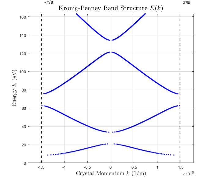
We solve the above equation using the following parameters, $a=3.9a_{bohr}$, $b=0.1a_{bohr}$, $V_0=-10$Ha, in the figure below, we take the energy $E_{min}=0$Ha while $E_{max}=6$Ha, we get:.
Ha is Hartrees, which exactly equal to 2 $Ry$ Rydberg, while 1$Ry$=13.6eV, is the famous energy ground state of the hydrogen atom.
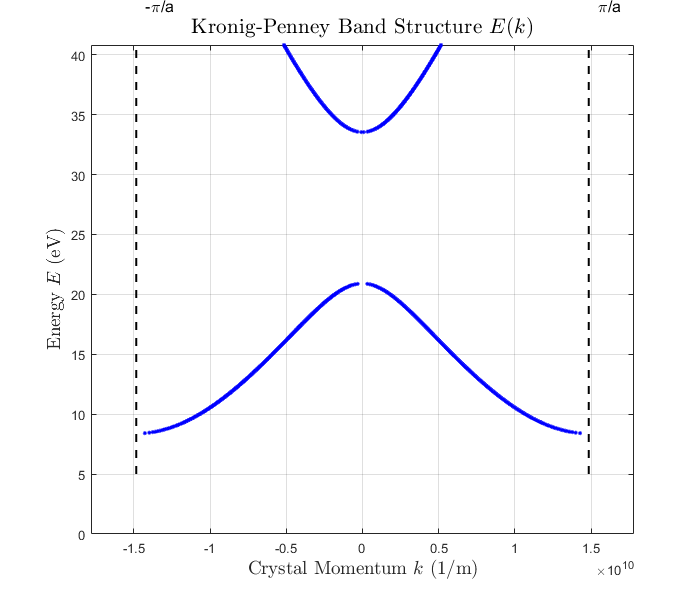
As we zoom in in the band structure diagram, we can crearly see the gap between the ground states band and the first exited states band, we do thzt by taking the energy interval $E_{min}=0$ while $E_{max}=1.5$Ha, we get:
§6 Physical Interpretation of Band Gaps
In the Kronig-Penney (KP) model, the band gaps appear so wide, there are two major physical reasons why a basic Kronig-Penney square potential naturally exaggerates and inflates the size of forbidden band gaps. The first one is the interstitial barrier height, because a rectangle fills up the entire interstitial space with maximum potential energy, the total area and "strength" of the barrier in the KP model is drastically larger. It acts like a heavy brick wall instead of a sloped hill, making it much harder for electrons to tunnel from one well to another. When tunneling decreases, the bands flatten out, and the forbidden gaps between them widen massively.
The second culprit are the high-frequency Fourier components (Bragg Reflection Strength), because the step edges are infinitely sharp, high-energy electrons experience incredibly strong quantum mechanical back-scattering (Bragg reflection) off those vertical walls. This keeps the gaps wide even when you go high up in energy.
§7 The 1D Hydrogen Chain: Beyond Square Wells
While the Kronig–Penney model is exactly solvable and pedagogically invaluable, its square-well potential is a drastic approximation. A hydrogen atom creates a Coulomb potential $V(x) = -e^2 / (4\pi\epsilon_0 |x|)$, which has a cusp at $x = 0$ and long algebraic tails. In a one-dimensional chain of hydrogen atoms with spacing $d$, the total potential is
We focus on a single-atom cell of width $a$ centred at the origin, which has three distinct regions (see Fig. 2):
Central region ($|x| < a/2$, green): the potential is nearly flat for small $|x|$ but contains the Coulomb singularity. Right Coulomb tail ($x > a/2$): the potential decays as $-e^2/x$. Left Coulomb tail ($x < -a/2$): the potential decays as $+e^2/x$ (from the atom in the next cell to the left).
§8 Whittaker Functions and the Coulomb Solution
In the central region, the wavefunction can be written as plane waves (assuming a locally flat effective potential approximation):
However, in the Coulomb tail regions, the Schrödinger equation takes the Whittaker form. For a particle with energy $E < 0$ (bound-state band) the Schrödinger equation in the right tail region $x > 0$ reads
Setting $\rho = 2k_r x$ with $k_r = \sqrt{-2mE}/\hbar$ and $n = e^2/(4\pi\epsilon_0 \hbar^2 k_r / m)$ as the effective principal quantum number, this transforms into Whittaker's equation. The two independent solutions are the Whittaker $M$ and $W$ functions:
where $M_{\kappa,\mu}(z)$ grows exponentially for large $z$ and $W_{\kappa,\mu}(z)$ decays exponentially. In an infinite crystal, neither solution can be discarded — both are needed to match the Bloch boundary conditions across the cell.
For the left tail ($x < 0$), the Hamiltonian takes this form:
The argument for choosing this form is to keep the core of the equation consistent with our primary goal: solving for an attractive Coulomb potential. By preserving this form, the negative values of $x$ will cancel out with the negative sign introduced in the Hamiltonian, restoring the attractive Coulomb potential for $x < 0$. The resulting solutions take the following form:
§9 Transfer-Matrix Formulation for the H-Chain
We construct the state vectors $\Omega_{\rm region}(x)$ for each zone, analogous to those used in the Kronig–Penney case. Specifically, we collect the wavefunction and its derivative into a column vector and define the Whittaker fundamental matrix:
and similarly for $\Omega_l(x)$ (with $k_r \to k_l$ and $x \to -x$). The boundary conditions at $x = \pm a/2$ are then expressed compactly as:
The boundary conditions at $x = \pm c$ are then expressed compactly as:
Eliminating the central-region amplitudes $(A, B)$, $(C, D)$ and $(E, F)$ between these two equations gives a direct relation between the left-tail amplitudes $(\psi\left(-\tfrac{a}{2}\right), \psi'\left(-\tfrac{a}{2}\right))$ and the right-tail amplitudes $(\psi\left(\tfrac{a}{2}\right), \psi'\left(\tfrac{a}{2}\right))$:
The matrix $\mathbf{T}_{\rm H}$ is the hydrogen-chain transfer matrix. Its trace furnishes the dispersion relation via the same Bloch condition as before:
where $d$ is the lattice constant (inter-atomic spacing). The numerical evaluation of $\mathbf{T}_{\rm H}$ requires computing Whittaker functions and their derivatives — a task straightforwardly handled by standard scientific computing libraries (SciPy, GSL).
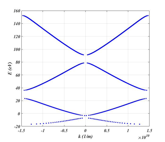
We solve the above equation using the following parameters, $Z=1$, $a=4a_{bohr}$, $c=0.1a_{bohr}$, $V_0=-10$Ha, in the figure below, we take the energy $E_{min}=-2$Ha while $E_{max}=6$Ha, we get:.
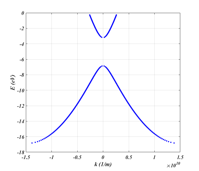
We use the same parameters but we decrease the energy interval by taking the energy $E_{min}=-2$Ha while $E_{max}=-0.01$Ha, we get the following:
§10/span> Comparison and Physical Consequences
Both models obey the same underlying mathematical framework: Bloch's theorem, boundary matching, and the trace condition $\text{Tr}(\mathbf{T}) = 2\cos(kd)$. Their differences reflect the physics of the potential:
| Feature | Kronig–Penney | H-Chain |
|---|---|---|
| Potential shape | Square well/barrier | Coulomb $\sim 1/|x|$ |
| Zone solutions | Plane waves $e^{\pm ik_j x}$ | Whittaker $M_n$, $W_n$ |
| Dispersion relation | Analytic (closed form) | Numerical ($\text{Tr}\,\mathbf{T}_H$) |
| Isolated-atom limit | Particle-in-a-box levels | Hydrogen levels $E_n$ |
| Band-gap mechanism | Bragg reflection at BZ boundary | Same + Coulomb-level splitting |
The hydrogen chain predicts narrower bands and larger gaps for the lowest bands, owing to the stronger localisation of Coulomb-bound states compared to square-well states. For higher bands (large $n$), the hydrogen wavefunctions extend further, the Whittaker functions approach Bessel functions, and the two models converge.
These models form the conceptual backbone of modern density-functional theory (DFT): the Kohn–Sham equations reduce the many-body problem to a set of single-particle Schrödinger equations in an effective periodic potential, and the resulting band structure determines conductivity, optical absorption, magnetism, and superconductivity. The transfer-matrix technique, in its layered form, is also the basis of modern photonic bandgap calculations and quantum cascade laser design.
References
- Kronig, R. de L. & Penney, W. G. (1931). Quantum Mechanics of Electrons in Crystal Lattices. Proceedings of the Royal Society A, 130(814), 499–513.
- Kittel, C. (2005). Introduction to Solid State Physics, 8th ed. Wiley.
- Ashcroft, N. W. & Mermin, N. D. (1976). Solid State Physics. Holt, Rinehart & Winston.
- Abramowitz, M. & Stegun, I. A. (1972). Handbook of Mathematical Functions. Dover. §13 (Whittaker Functions).
- Griffiths, D. J. (2018). Introduction to Quantum Mechanics, 3rd ed. Cambridge University Press.
- Bloch, F. (1929). Über die Quantenmechanik der Elektronen in Kristallgittern. Zeitschrift für Physik, 52, 555–600.